About

When I’m not working my day job as a software developer, I enjoy learning about history, exploring open-source and self-hosted technologies, and appreciating pixel art.

Work Experience

Software Developer (June, 2024 - June, 2025)

As a Full Stack Developer at CCRPC (Champaign County Regional Planning Commission):

ILGISA 2025 Chicago Regional Conference

• Solve Problems, Build Tools, Save Money

ILGISA 2024 Annual Conference

• Open Source GIS Workflows on a Linux Desktop

Census Downloader

The U.S. Census Bureau’s data and geographical boundaries are accessible through two different APIs. Traditionally, planners had to manually join these two tables using their GEOIDs—a process that was time-consuming, required Python scripting knowledge, and was complicated by inconsistent GEOID formats across datasets.

I was tasked with developing a QGIS Plugin that automatically combined Census data and geographical boundaries through a clean, user-friendly GUI. The original codebase contained over 3,000 lines and suffered from limited functionality, poor extensibility, and exposed API keys. By rewriting it, I reduced the codebase to under 1,000 lines while improving performance, functionality, and extensibility.

Background

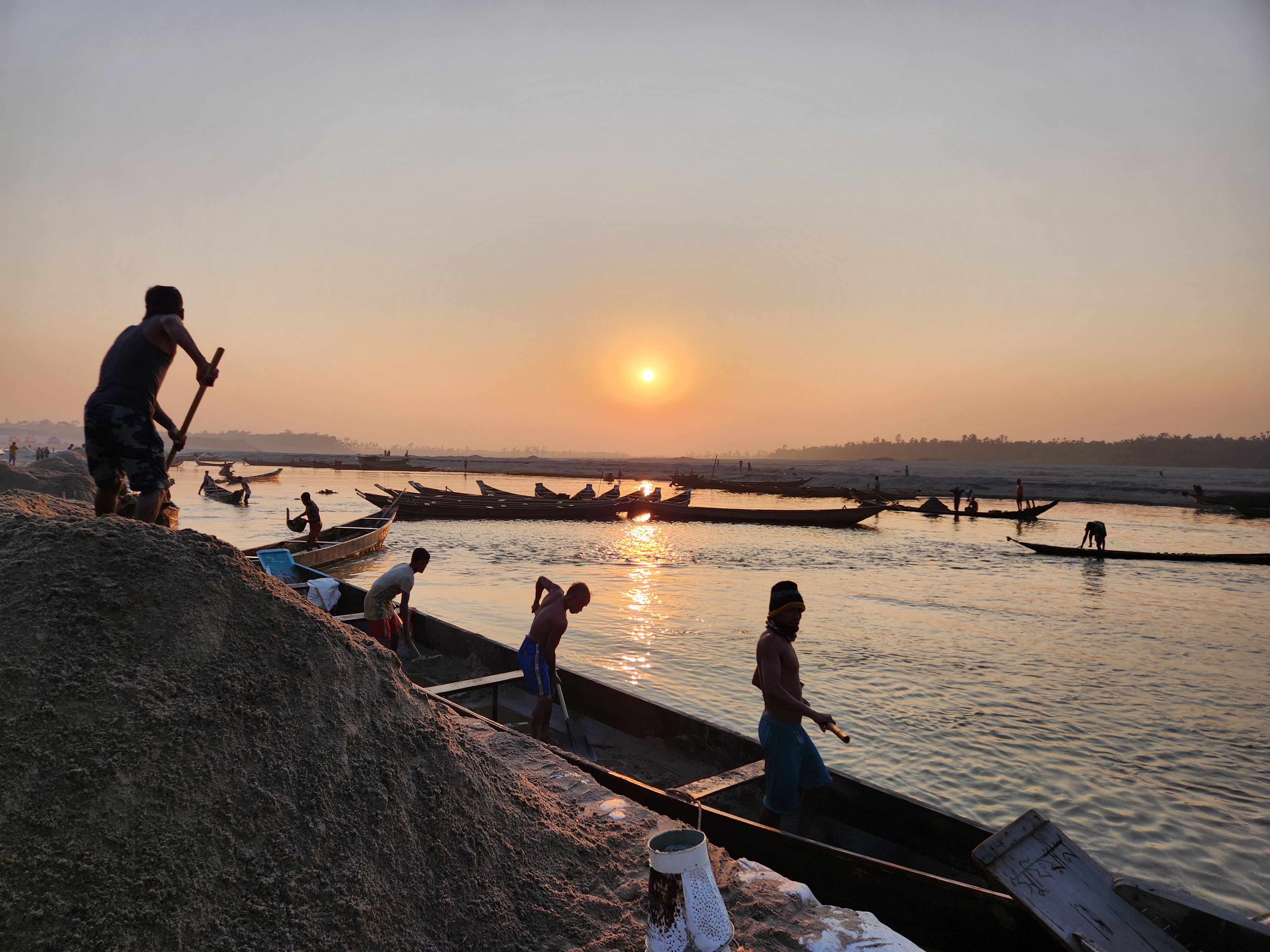
Sand and gravel are two highly sought-after raw materials in the global market. Coarse sand dredged from rivers is used in semiconductor and glass manufacturing. Finer sand is in high demand for wetland reclamation, which is important for expanding infrastructure in areas affected by climate change. Gravel is a crucial material for both concrete and asphalt production. Flowing from the Himalayas into the Gangetic Plain, the Brahmaputra deposits coarse silt and gravel directly into the Bengal Basin.

Flood Risk Calculation

# Load necessary packages
library(raster)
library(rasterVis)
library(maptools)
library(rgdal)
# Set working directory
setwd("<YOUR DIRECTORY>")

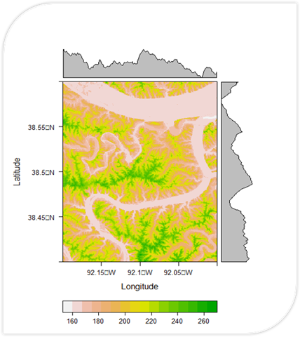
# Load DEM file
dem <- raster("RiverUSGS.tif")

plot(dem)

# Plot DEM map
plot(dem, col = rev(terrain.colors(50)))

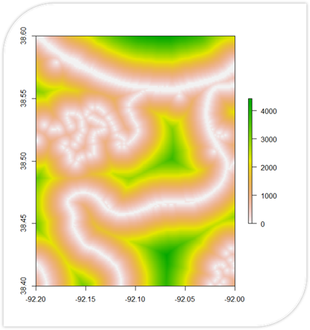
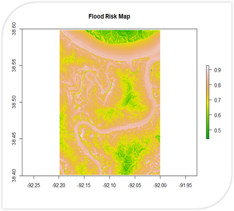
# Set extent for cropping
ext <- extent(-92.2, -92.0, 38.4, 38.6)

# Crop DEM to desired extent
demnew <- crop(dem, ext)

plot(demnew)
# Plot cropped DEM map
plot(demnew, col = rev(terrain.colors(50)))

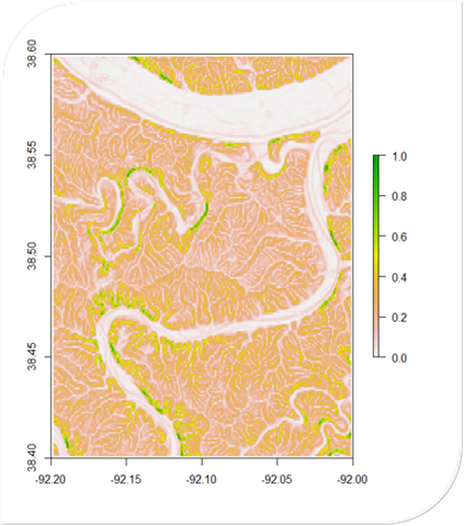
# Extract elevation values at each cell
elevations <- getValues(demnew)

# Calculate flood risk
flood_risk <- (1 - (elevations / max(elevations)))

# Create raster object for flood risk layer
flood_risk_raster <- raster(demnew)
values(flood_risk_raster) <- flood_risk

# Define custom color palette for flood risk map
my_palette <- colorRampPalette(c("yellow", "red"))

# Plot DEM map with custom color palette
levelplot(demnew, col.regions = rev(terrain.colors(50)))

# Add flood risk map with custom color palette
floodriskplot <- levelplot(flood_risk_raster, alpha = 0.5, add = TRUE, col.regions = my_palette(100))

floodriskplot

library(sf)

boundary <- st_read("Addresses.shp")

flood_data <- read.csv("flood_data.csv")
plot(flood_data$Height, flood_data$Discharge)

df2 <- data.frame(discharge = flood_data$Discharge, height = flood_data$Height)


# Save flood risk map
writeRaster(flood_risk_raster, "flood_risk.tif", format = "GTiff", overwrite = TRUE)


df <- data.frame(Elevation = elevations, Flood_Risk = flood_risk)

# Create a line chart to show the relationship between elevation and flood risk
plot(df$Elevation, df$Flood_Risk, type = "l", xlab = "Elevation", ylab = "Flood Risk", main = "Elevation vs Flood Risk")

noaa_data2 <- read.csv("RiverData2.csv")

A Flood Risk Calculator written in R. It uses DEM data to calculate slope and proximity (shown in their own respective maps). These are used to calculate a final flood risk assessment on a scale of 0 to 1.