School Projects
Flood Risk Calculation
# Load necessary packages
library(raster)
library(rasterVis)
library(maptools)
library(rgdal)
# Set working directory
setwd("<YOUR DIRECTORY>")
# Load DEM file
dem <- raster("RiverUSGS.tif")
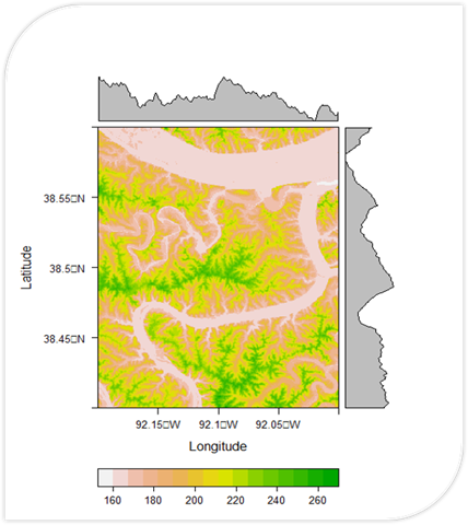
plot(dem)
# Plot DEM map
plot(dem, col = rev(terrain.colors(50)))
# Set extent for cropping
ext <- extent(-92.2, -92.0, 38.4, 38.6)
# Crop DEM to desired extent
demnew <- crop(dem, ext)
plot(demnew)
# Plot cropped DEM map
plot(demnew, col = rev(terrain.colors(50)))
# Extract elevation values at each cell
elevations <- getValues(demnew)
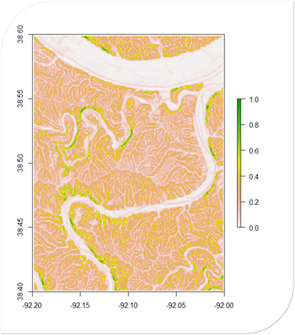
# Calculate flood risk
flood_risk <- (1 - (elevations / max(elevations)))
# Create raster object for flood risk layer
flood_risk_raster <- raster(demnew)
values(flood_risk_raster) <- flood_risk
# Define custom color palette for flood risk map
my_palette <- colorRampPalette(c("yellow", "red"))
# Plot DEM map with custom color palette
levelplot(demnew, col.regions = rev(terrain.colors(50)))
# Add flood risk map with custom color palette
floodriskplot <- levelplot(flood_risk_raster, alpha = 0.5, add = TRUE, col.regions = my_palette(100))
floodriskplot
library(sf)
boundary <- st_read("Addresses.shp")
flood_data <- read.csv("flood_data.csv")
plot(flood_data$Height, flood_data$Discharge)
df2 <- data.frame(discharge = flood_data$Discharge, height = flood_data$Height)
# Save flood risk map
writeRaster(flood_risk_raster, "flood_risk.tif", format = "GTiff", overwrite = TRUE)
df <- data.frame(Elevation = elevations, Flood_Risk = flood_risk)
# Create a line chart to show the relationship between elevation and flood risk
plot(df$Elevation, df$Flood_Risk, type = "l", xlab = "Elevation", ylab = "Flood Risk", main = "Elevation vs Flood Risk")
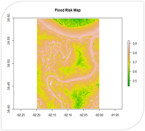
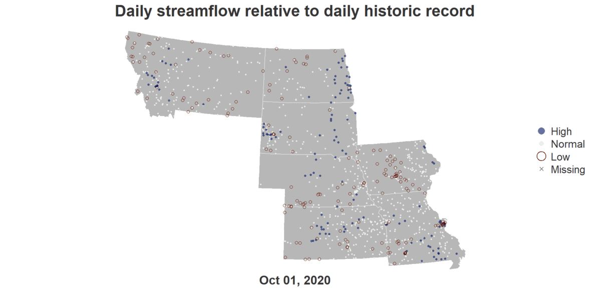
noaa_data2 <- read.csv("RiverData2.csv")A Flood Risk Calculator written in R. It uses DEM data to calculate slope and proximity (shown in their own respective maps). These are used to calculate a final flood risk assessment on a scale of 0 to 1.
Floodrisk of States Along Missouri River
install.packages("dataRetrieval")
install.packages("animation")
install.packages("maps")
install.packages("sf")
install.packages("magick")
install.packages("av")
library(dataRetrieval)
library(tidyverse) # includes dplyr, tidyr
library(maps)
library(sf)
library(magick)
library(av)

# Viz dates
viz_date_start <- as.Date("2020-10-01")
viz_date_end <- as.Date("2020-10-31")

# Currently set to CONUS (to list just a few, do something like `c("MN", "WI", "IA", "IL")`)
viz_states <- c("MT", "ND", "SD", "NE", "IA", "KS", "MO")

# Albers Equal Area, which is good for full CONUS
viz_proj <- "+proj=laea +lat_0=45 +lon_0=-100 +x_0=0 +y_0=0 +a=6370997 +b=6370997 +units=m +no_defs"

# Configs that could be changed ...
param_cd <- "00060" # Parameter code for streamflow . See `dataRetrieval::parameterCdFile` for more.
service_cd <- "dv" # means "daily value". See `https://waterservices.usgs.gov/rest/` for more info.

sites_available <- data.frame() # This will be table of site numbers and their locations.
for(s in viz_states) {
  # Some states might not return anything, so use `tryCatch` to allow
  # the `for` loop to keep going.
  message(sprintf("Trying %s ...", s))
  sites_available <- tryCatch(
    whatNWISsites(
      stateCd = s,
      startDate = viz_date_start,
      endDate = viz_date_end,
      parameterCd = param_cd,
      service = service_cd) %>%
      select(site_no, station_nm, dec_lat_va, dec_long_va),
    error = function(e) return()
  ) %>% bind_rows(sites_available)
}

head(sites_available)
# For one month of CONUS, this took ~ 15 min

# Can only pull stats for 10 sites at a time, so loop through chunks of 10
#   sites at a time and combine into one big dataset at the end!
sites <- unique(sites_available$site_no)

# Divide request into chunks of 10
req_bks <- seq(1, length(sites), by=10)

viz_stats <- data.frame()
for(chk_start in req_bks) {
  chk_end <- ifelse(chk_start + 9 < length(sites), chk_start + 9, length(sites))
  # Note that each call throws warning about BETA service :)
  message(sprintf("Pulling down stats for %s:%s", chk_start, chk_end))
  viz_stats <- tryCatch(readNWISstat(
    siteNumbers = sites[chk_start:chk_end],
    parameterCd = param_cd,
    statType = c("P25", "P75")
  ) %>% select(site_no, month_nu, day_nu, p25_va, p75_va),
  error = function(e) return()
  ) %>% bind_rows(viz_stats)
}

head(viz_stats)
# For all of CONUS, there are 8500+ sites.
# Just in case there is an issue, use a loop to cycle through 100
# at a time and save the output temporarily, then combine after.
# For one month of CONUS data, this took ~ 10 minutes

max_n <- 100
sites <- unique(sites_available$site_no)
sites_chunk <- seq(1, length(sites), by=max_n)
site_data_fns <- c()
tmp <- tempdir()

for(chk_start in sites_chunk) {
  chk_end <- ifelse(chk_start + (max_n-1) < length(sites),
                    chk_start + (max_n-1), length(sites))

  site_data_fn_i <- sprintf(
    "%s/site_data_%s_%s_chk_%s_%s.rds", tmp,
    format(viz_date_start, "%Y_%m_%d"), format(viz_date_end, "%Y_%m_%d"),
    # Add leading zeroes in front of numbers so they remain alphanumerically ordered
    sprintf("%02d", chk_start),
    sprintf("%02d", chk_end))
  site_data_fns <- c(site_data_fns, site_data_fn_i)

  if(file.exists(site_data_fn_i)) {
    message(sprintf("ALREADY fetched sites %s:%s, skipping ...", chk_start, chk_end))
    next
  } else {
    site_data_df_i <- readNWISdata(
      siteNumbers = sites_available$site_no[chk_start:chk_end],
      startDate = viz_date_start,
      endDate = viz_date_end,
      parameterCd = param_cd,
      service = service_cd
    ) %>% renameNWISColumns() %>%
      select(site_no, dateTime, Flow)
    saveRDS(site_data_df_i, site_data_fn_i)
    message(sprintf("Fetched sites %s:%s out of %s", chk_start, chk_end, length(sites)))
  }

}

# Read and combine all of them
viz_daily_values <-  lapply(site_data_fns, readRDS) %>% bind_rows()

nrow(viz_daily_values) # ~250,000 obs for one month of CONUS data

head(viz_daily_values)
# To join with the stats data, we need to first break the dates into
# month day columns
viz_daily_stats <- viz_daily_values %>%
  mutate(month_nu = as.numeric(format(dateTime, "%m")),
         day_nu = as.numeric(format(dateTime, "%d"))) %>%
  # Join the statistics data and automatically match on month_nu and day_nu
  left_join(viz_stats) %>%
  # Compare the daily flow value to that sites statistic to
  # create a column that says whether the value is low, normal, or high
  mutate(viz_category = ifelse(
    Flow <= p25_va, "Low",
    ifelse(Flow > p25_va & Flow <= p75_va, "Normal",
           ifelse(Flow > p75_va, "High",
                  NA))))

head(viz_daily_stats)
# Viz frame height and width. These are double the size the end video &
#   gifs will be. See why in the "Optimizing for various platforms" section
viz_width <- 2048 # in pixels
viz_height <- 1024 # in pixels

# Style configs for plotting (all are listed in the same order as the categories)
viz_categories <- c("High", "Normal", "Low", "Missing")
category_col <- c("#00126099", "#EAEDE9FF", "#601200FF", "#7f7f7fFF") # Colors (hex + alpha code)
category_pch <- c(16, 19, 1, 4) # Point types in order of categories
category_cex <- c(1.5, 1, 2, 0.75) # Point sizes in order of categories
category_lwd <- c(NA, NA, 1, NA) # Circle outline width in order of categories
# Created a function to use that picks out the correct config based on
# category name. Made it a fxn since I needed to do it for colors,
# point types, and point sizes. This function assumes that all of the
# config vectors are in the order High, Normal, Low, and Missing.
pick_config <- function(viz_category, config) {
  ifelse(
    viz_category == "Low", config[3],
    ifelse(viz_category == "Normal", config[2],
           ifelse(viz_category == "High", config[1],
                  config[4]))) # NA color
}

# Add style information as 3 new columns
viz_data_ready <- viz_daily_stats %>%
  mutate(viz_pt_color = pick_config(viz_category, category_col),
         viz_pt_type = pick_config(viz_category, category_pch),
         viz_pt_size = pick_config(viz_category, category_cex),
         viz_pt_outline = pick_config(viz_category, category_lwd)) %>%
  # Simplify columns
  select(site_no, dateTime, viz_category, viz_pt_color,
         viz_pt_type, viz_pt_size, viz_pt_outline) %>%
  left_join(sites_available) %>%
  # Arrange so that NAs are plot first, then normal values on top of those, then
  # high values, and then low so that viewer can see the most points possible.
  arrange(dateTime, factor(viz_category, levels = c(NA, "Normal", "High", "Low")))

# Convert to `sf` object for mapping
viz_data_sf <- viz_data_ready %>%
  st_as_sf(coords = c("dec_long_va", "dec_lat_va"), crs = "+proj=longlat +datum=WGS84") %>%
  st_transform(viz_proj)

head(viz_data_sf)
# Convert state codes into lowercase state names, which `maps` needs
viz_state_names <- tolower(stateCdLookup(viz_states, "fullName"))
state_sf <- st_as_sf(maps::map('state', viz_state_names, fill = TRUE, plot = FALSE)) %>%
  st_transform(viz_proj)

head(state_sf)
png("test_single_day.png", width = viz_width, height = viz_height)

# Prep plotting area (no outer margins, small space at top/bottom for title, white background)
par(omi = c(0,0,0,0), mai = c(0.5,0,0.5,0.25), bg = "white")

# Add the background map
plot(st_geometry(state_sf), col = "#b7b7b7", border = "white")

# Add gages for the first day in the data set
viz_data_sf_1 <- viz_data_sf %>% filter(dateTime == viz_date_start)
plot(st_geometry(viz_data_sf_1), add=TRUE, pch = viz_data_sf_1$viz_pt_type,
     cex = viz_data_sf_1$viz_pt_size, col = viz_data_sf_1$viz_pt_color,
     lwd = viz_data_sf_1$viz_pt_outline)

# Now add on a title, the date, and a legend
text_color <- "#363636"
title("Daily streamflow relative to daily historic record", cex.main = 4.5, col.main = text_color)
mtext(format(viz_date_start, "%b %d, %Y"), side = 1, line = 0.5, cex = 3.5, font = 2, col = text_color)
legend("right", legend = viz_categories, col = category_col, pch = category_pch,
       pt.cex = category_cex*3, pt.lwd = category_lwd*2, bty = "n", cex = 3, text.col = text_color)

dev.off()
# This takes ~2 minutes to create a frame per day for a month of data

frame_dir <- "frame_tmp" # Save frames to a folder
frame_configs <- data.frame(date = unique(viz_data_sf$dateTime)) %>%
  # Each day gets it's own file
  mutate(name = sprintf("%s/frame_%s.png", frame_dir, date),
         frame_num = row_number())

if(!dir.exists(frame_dir)) dir.create(frame_dir)

# Loop through dates
for(i in frame_configs$frame_num) {
  this_date <- frame_configs$date[i]

  # Filter gage data to just this day:
  data_this_date <- viz_data_sf %>% filter(dateTime == this_date)

  png(frame_configs$name[i], width = viz_width, height = viz_height) # Open file

  # Copied plotting code from previous step
  # Prep plotting area (no outer margins, small space at top/bottom for title, white background)
  par(omi = c(0,0,0,0), mai = c(1,0,1,0.5), bg = "white")

  # Add the background map
  plot(st_geometry(state_sf), col = "#b7b7b7", border = "white")

  # Add gages for this day
  plot(st_geometry(data_this_date), add=TRUE, pch = data_this_date$viz_pt_type,
       cex = data_this_date$viz_pt_size, col = data_this_date$viz_pt_color,
       lwd = data_this_date$viz_pt_outline)

  # Add the title, date, and legend
  text_color <- "#363636"
  title("Daily streamflow relative to daily historic record",
        cex.main = 4.5, col.main = text_color)
  mtext(format(this_date, "%b %d, %Y"), side = 1, line = 0.5,
        cex = 3.5, font = 2, col = text_color)
  legend("right", legend = viz_categories, col = category_col,
         pch = category_pch, pt.cex = category_cex*3,
         pt.lwd = category_lwd*2, bty = "n", cex = 3,
         text.col = text_color)

  dev.off() # Close file
}

# You can check that all the files were created by running
all(file.exists(frame_configs$name))

# GIF configs that you set
frames <- frame_configs$name # Assumes all are in the same directory
gif_length <- 10 # Num seconds to make the gif
gif_file_out <- sprintf("animation_%s_%s.gif",
                        format(viz_date_start, "%Y_%m_%d"),
                        format(viz_date_end, "%Y_%m_%d"))

# ImageMagick needs a temporary directory while it is creating the GIF to
#   store things. Make sure it has one. I am making this one, inside of
#   the directory where our frames exist.
tmp_dir <- sprintf("%s/magick", dirname(frames[1]))
if(!dir.exists(tmp_dir)) dir.create(tmp_dir)

# Calculate GIF delay based on desired length & frames
# See https://legacy.imagemagick.org/discourse-server/viewtopic.php?t=14739
fps <- length(frames) / gif_length # Note that some platforms have specific fps requirements
gif_delay <- round(100 / fps) # 100 is an ImageMagick default (see that link above)

# Create a single string of all the frames going to be stitched together
#   to pass to ImageMagick commans.
frame_str <- paste(frames, collapse = " ")

# Create the ImageMagick command to convert the files into a GIF
magick_command <- sprintf(
  'convert -define registry:temporary-path=%s -limit memory 24GiB -delay %s -loop 0 %s %s',
  tmp_dir, gif_delay, frame_str, gif_file_out)

# If you are on a Windows machine, you will need to have `magick` added before the command
if(Sys.info()[['sysname']] == "Windows") {
  magick_command <- sprintf('magick %s', magick_command)
}

# Now actually run the command and create the GIF
system(magick_command)

setwd("<YOUR FILE PATH>")

# Get the list of PNG files
png_files <- list.files(pattern = "\\.png$")

# Sort the file names in ascending order
png_files <- sort(png_files)

# Read the PNG files and combine them into a single GIF
gif <- image_read(png_files)
image_write(gif, "output.gif")
# Get list of PNG files
png_files <- list.files(pattern = "\\.png$")

# Sort files in ascending order
png_files <- sort(png_files)

# Read PNGs and add them to GIF frame by frame
gif <- image_read(png_files)
gif
image_write(gif, "output.gif")
An R script that generates a GIF showing Flood Risks of cities in the Missouri River Basin across October of 2020.
Forest Park Missouri
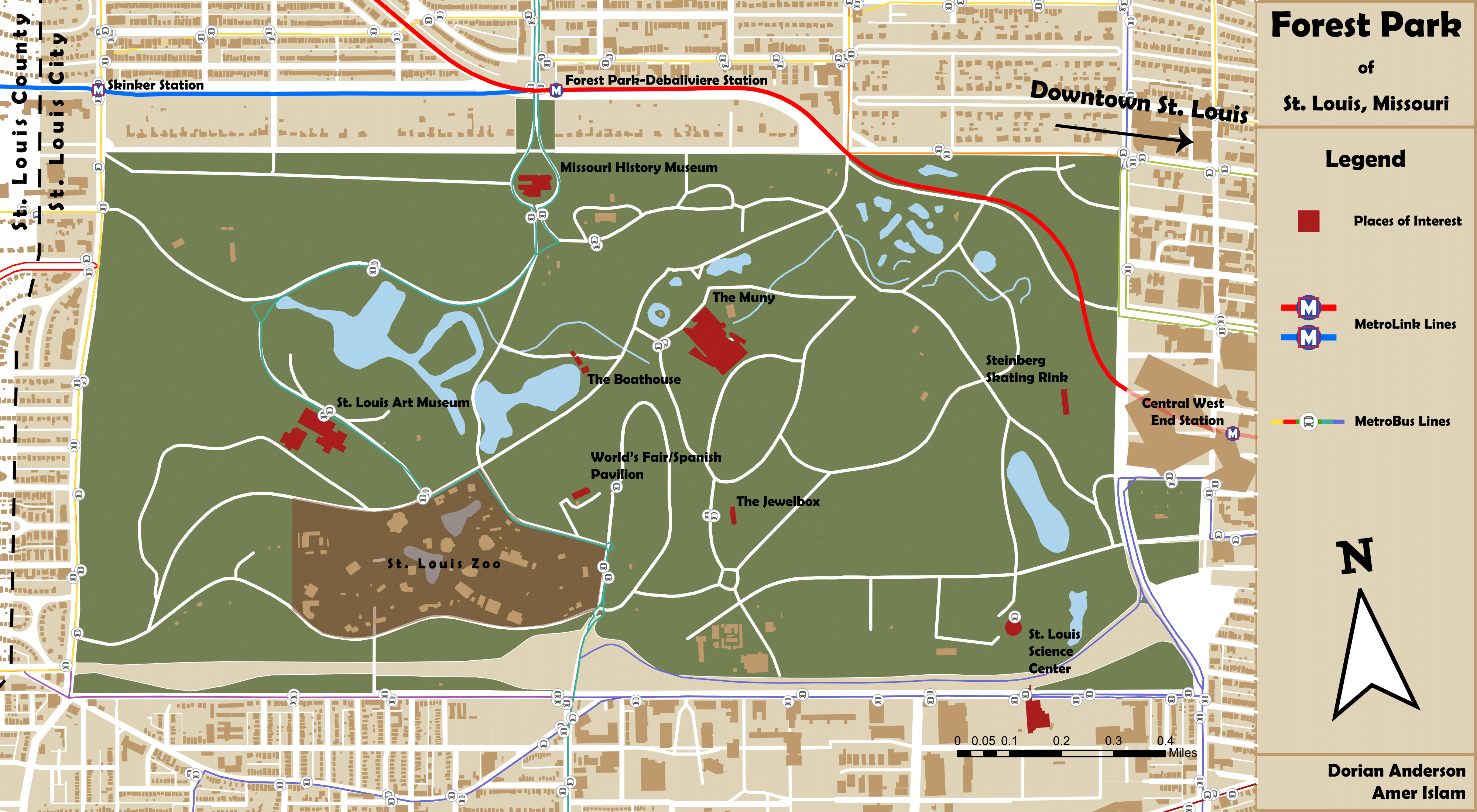
A mock Tourist map for Forest Park in St. Louis, MO.
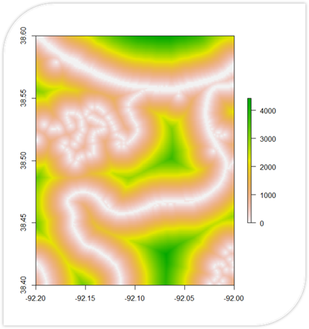
Grand Canyon DEM
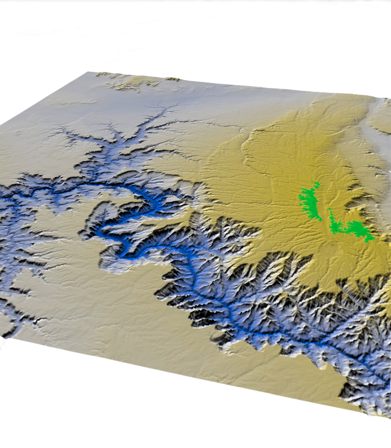
Using USGS Elevation Data, I created a Digital Elevation Model of the Grand Canyon in Arizona. Greener hues indicate higher altitudes, while bluer hues represent lower elevations.
Rural Hospital Closures
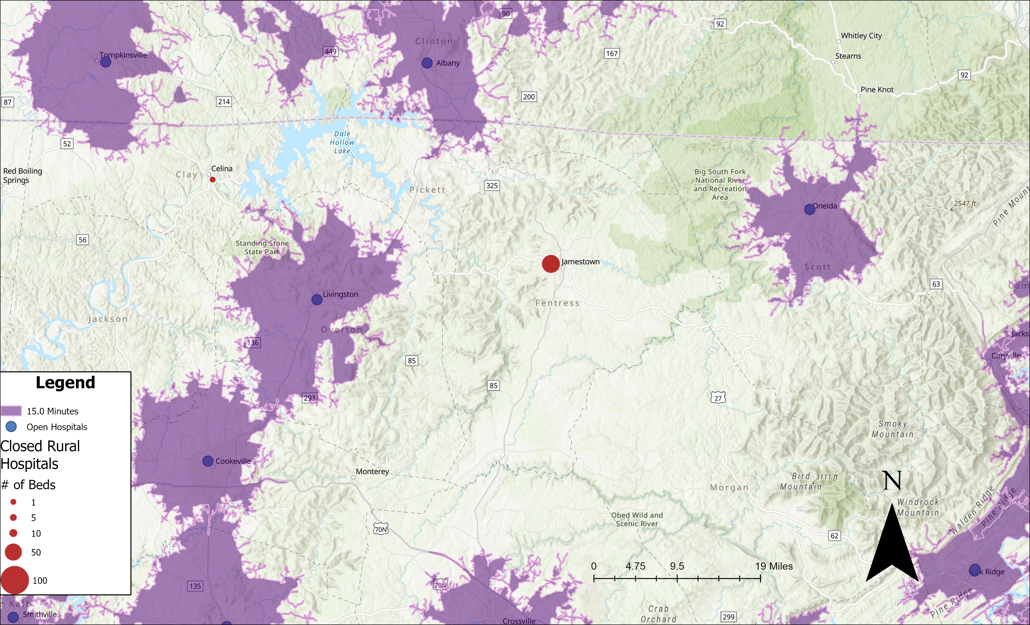
In recent years, hospital closures have swept across the American Heartland. Here, we focus on Jamestown, Tennessee—a small town with a population under 2,000 that recently lost its hospital. Nestled between a mountain range and nature preserves, residents now find themselves more than a 15‑minute drive from the nearest hospital.